Two-Way-ANOVA

In data analysis, it’s common to ask whether one factor influences an outcome — for example, does the quarter of the year affect sales? That’s where one-way ANOVA comes in. But business problems are rarely that simple. Sales may not only depend on the quarter but also on other factors, like region, marketing strategy, or product category.

If we only look at one factor, we risk missing the bigger picture. That’s where two-way ANOVA becomes useful. It lets us test the effect of two independent factors at the same time, and more importantly, whether there’s an interaction between them.

Take our sales example:

• One factor is the quarter (Q1, Q2, Q3, Q4).
• Another factor is the region (say, East and West).

Using two-way ANOVA, we can analyze:

• The effect of quarter on sales.
• The effect of region on sales.
• The interaction effect — do some quarters perform better in one region than another?

Let's extend the same quarterly sales example we used in one-way ANOVA. Previously, we tested whether sales varied across quarters. Now, we will introduce a second factor "region", to explore whether sales patterns differ not just by quarter, but also by geography, and whether the two factors interact.

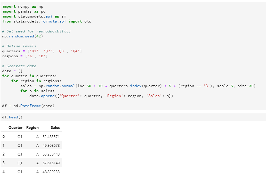
We’ll simulate sales data for:

• 4 Quarters: Q1, Q2, Q3, Q4
• 2 Regions: Region A and Region B
• 30 observations per group → Total: 4 × 2 × 30 = 240 rows

Each row will have:

• Quarter (categorical)
• Region (categorical)
• Sales (numeric)

Key Parameters in Two-Way ANOVA Output

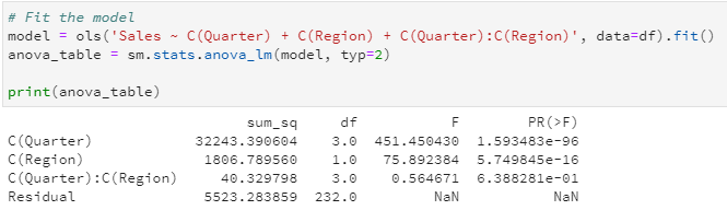
1. sum_sq (Sum of Squares)

   • Measures the variation in sales explained by each factor (Quarter, Region, Interaction).

   • Larger values mean that factor explains more of the variation in sales.

2. df (Degrees of Freedom)

   • Related to how many groups or categories the factor has.

   • Example: 4 quarters → 3 degrees of freedom (always groups − 1).

3. F (F-statistic)

   • Ratio of the variation explained by the factor to the unexplained variation (error).

   • Higher F = stronger evidence that the factor significantly affects the outcome.

4. PR(>F) (p-value)

   • Probability of seeing these results if the null hypothesis (no effect) were true.

   • Small p-value (usually < 0.05) → the factor has a statistically significant effect.

5. Residual

   • The leftover variation in sales that can’t be explained by Quarter, Region, or their interaction.

   • Think of it as “random noise” or unmeasured factors.

Let’s break down the result of Two-Way ANOVA test step by step in simple terms:

1. C(Quarter)

• F = 451.45, p-value ≈ 1.59e-96 (basically 0)
• This means Quarter has a huge and highly significant effect on Sales.
• In plain words: Sales are not the same across quarters — the quarter of the year strongly influences sales.

2. C(Region)

• F = 75.89, p-value ≈ 5.75e-16 (again, almost 0)
• Region also has a strong, statistically significant effect.
• Translation: Sales differ significantly between regions.

3. C(Quarter):C(Region) (Interaction effect)

• F = 0.56, p-value ≈ 0.638 (greater than 0.05)
• This means the interaction effect is not significant.
• In business terms: The way sales vary across quarters is similar in both regions. No special quarter-region combination stands out as unusual.

4. Residual (Error)

• This is just the variation in Sales that isn’t explained by Quarter, Region, or their interaction.

Overall, both Quarter and Region individually affect sales. But the combination of Quarter and Region doesn’t matter much — sales differences between quarters look roughly the same in all regions.