Loan Approval(Logistic Regression)

In this project, we explore predictive analytics in the context of loan approvals. Our goal is to understand the factors influencing approval decisions and assess how accurately we can predict them. We begin by examining the dataset and uncovering patterns through targeted visualizations. These insights then guide us into building a logistic regression model, allowing us to quantify relationships and evaluate the model’s predictive power.

The data has been picked from kaggle: https://www.kaggle.com/datasets/abhishekmishra08/loan-approval-datasets?resource=download&select=loan_data.csv

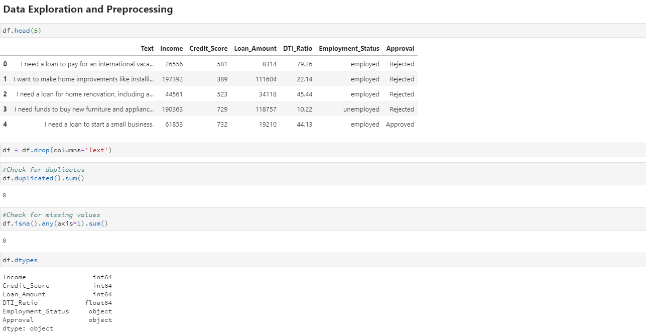
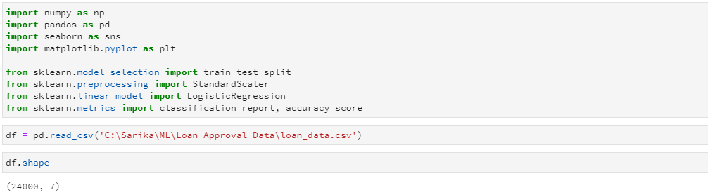
Let's import the libraries and read the source file. There are 24,000 rows in the file.

Now, let's explore the dataset and perform preprocessing if needed. We'll check for and remove any duplicate rows or missing values to ensure data quality before moving into analysis.

Let's see what story is each of the above visual telling us.

  • Employment Status vs Approval (Bar Plot)

This plot shows loan approval outcomes across employment categories. All approved loans belong to employed individuals, while unemployed applicants receive no approvals at all. It highlights employment status as a strong categorical predictor.

  • Income vs Loan Amount by Approval (Scatter Plot)

This scatter plot reveals a proportional relationship between income and loan amount. Approved loans tend to cluster within a balanced range, while rejected ones show more dispersion. It suggests financial scale and proportionality influence approval decisions.

  • DTI Ratio Distribution by Approval (Histogram)

This visualization compares the distribution of DTI ratios for approved and rejected loans. Rejected applications skew toward higher DTI values, while approved ones concentrate at lower ratios. It indicates DTI is a key differentiator in approval outcomes.

  • DTI Ratio by Approval (Boxplot)

The boxplot shows that the median DTI ratios for approved and rejected loans are quite similar. However, rejected loans exhibit greater dispersion with numerous outliers, indicating higher variability. This pattern reinforces the significance of DTI as a key factor influencing loan approval decisions.

Modeling Approach

Our target variable, loan approval, is binary—either "Approved" or "Rejected"—making logistic regression an ideal choice. 

While the dataset includes a Text column describing loan purpose, it contains unstructured data that cannot be meaningfully quantified without natural language processing techniques such as tokenization or sentiment analysis. Including it without proper preprocessing would introduce noise and risk degrading model performance. Logistic regression also requires all input features to be numeric. To meet this requirement, we’ll drop the Text column and apply encoding techniques to convert categorical variables—specifically Approval and Employment_Status—into numerical form. This ensures compatibility with the model. 

To assess how well our logistic regression model generalizes to unseen data, we’ll begin by splitting the dataset into training and test sets. The training set will be used to fit the model, while the test set provides an unbiased evaluation of its predictive performance. Once the model is trained, we’ll generate predictions on the test data and evaluate them using key classification metrics. These include accuracy, precision, recall, and the confusion matrix—all of which help us understand how effectively the model distinguishes between approved and rejected loan applications.

Interpretation

Accuracy: The model correctly predicted ~93% of all loan approval outcomes showing strong overall performance.

Precision: When the model predicts “Approved,” it’s correct ~78% of the time - meaning it does not make too many false approvals.

Recall: The model successfully captures around 77% of all actual approvals, though it misses a few genuine ones. 

F1 Score: The F1 score of 0.78 shows a good balance between precision and recall, which is important when approval and rejection cases are not equally represented.


Interpretation

  • True Negatives (5822): These are correctly predicted rejections—your model is very strong at identifying non-approved cases.
  • True Positives (877): These are correctly predicted approvals—your model is also solid at identifying approved cases.
  • False Positives (246): These are cases where the model incorrectly predicted approval for someone who was actually rejected. Very low—great precision.
  • False Negatives (255): These are missed approvals—cases where the model predicted rejection but the loan was actually approved. This is the main source of error.

Conclusion

The model demonstrates strong overall performance, accurately predicting about 93% of loan approval outcomes. It effectively distinguishes between approved and rejected cases, with a particularly high ability to identify non-approved loans (True Negatives).

While precision (78%) and recall (77%) indicate balanced performance, the few missed approvals (False Negatives) suggest that the model could be slightly improved to better capture borderline approval cases.

Overall, the results show that the model is reliable, well-balanced, and practical for deployment in predicting loan approval decisions, with room for fine-tuning to further enhance recall.