One-Way ANOVA(​Analysis of Variance)

When working with data, we often want to compare more than two groups. 

  • For example: Do students from different schools score the same on an exam? 
  • Do three marketing campaigns lead to the same average sales? 
  • Do four different diets result in the same average weight loss? 

If you only had two groups, you could use a t-test. But what if you have three or more groups? Running multiple t-tests isn’t a good idea. This is where One-Way ANOVA comes in. “ANOVA” stands for Analysis of Variance, because the test works by comparing variation between groups to variation within groups. 

What is One-Way ANOVA?

One-Way ANOVA is a statistical test used to compare the means of three or more independent groups to see if at least one group’s mean is significantly different from the others. 

“One-Way” means there’s only one factor (independent variable) that defines the groups. 

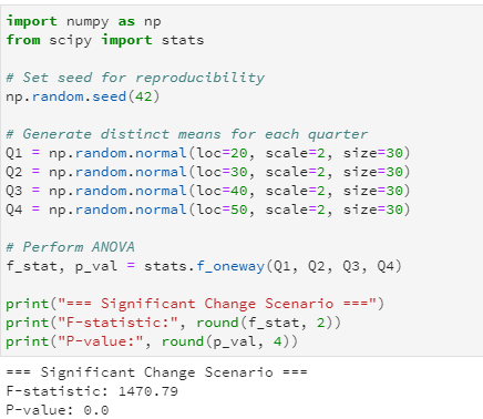
Example: "Quarter" when comparing quarterly sales.

How Does it Work?

Between-Group Variation → Measures how much the group means differ from the overall mean.

Within-Group Variation → Measures how much individual data points vary within each group. 

If the differences between groups are large compared to the differences within groups, then at least one group mean is likely different. 

Hypotheses in One-Way ANOVA

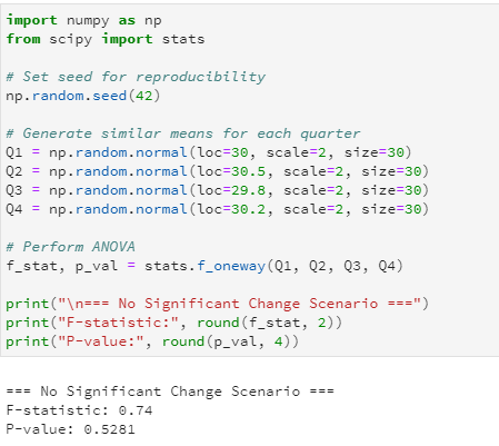
Null Hypothesis (H₀): All group means are equal. 

Example: Average sales are the same in all four quarters. 


Alternative Hypothesis (H₁): At least one group mean is different. 

Example: At least one quarter’s sales are different from the others.


Let’s walk through a hands-on example using Python to illustrate how One-Way ANOVA works in practice.

We’ll simulate two scenarios:

  1. Clear Differences Between Groups — where we expect to reject the null hypothesis.
  2. Subtle Differences — where the variation is small and we likely fail to reject the null.

Scenario 1: Significant change across quarters

We’ll use numpy.random.normal() to generate synthetic data. This function creates normally distributed numbers based on:

  • loc: the mean of the distribution
  • scale: the standard deviation (spread)
  • size: the number of values to generate

What’s Happening Here?

  • Each quarter has a distinct average: 20, 30, 40, and 50.
  • The standard deviation is small (±2), so the data within each group is tightly clustered.
  • The ANOVA test compares the between-group variance (differences in means) to the within-group variance (spread inside each group).

Expected Outcome

Because the group means are far apart and the data is tightly clustered, the between-group variance dominates. This leads to:

  • A high F-statistic
  • A low p-value (typically < 0.05)

This means we reject the null hypothesis and conclude that at least one quarter’s sales are significantly different.

Scenario 2: No significant change across quarters

What’s Different This Time?

  • The group means are very close: 30, 30.5, 29.8, and 30.2.
  • The standard deviation is still ±2, so the data within each group is similarly spread.
  • Because the group averages are nearly the same, the between-group variation is small.

Expected Outcome

In this case, the ANOVA test will likely return:

  • A low F-statistic
  • A high p-value (typically > 0.05)

This means we fail to reject the null hypothesis, concluding that there’s no statistically significant difference in sales across quarters.

This scenario shows how One-Way ANOVA helps avoid false conclusions. Even if the numbers look slightly different, ANOVA tells us whether those differences are statistically meaningful or just random variation.

What Happens After ANOVA?

One-Way ANOVA is powerful—but it only tells you that a difference exists among the group means. It doesn’t tell you where that difference lies.

Let’s say your ANOVA test returns a significant result (p-value < 0.05). That means at least one group is different—but which one? Is Q2 higher than Q1? Is Q4 different from Q3? To answer that, you need a post-hoc test.

What is Post-Hoc Test?

Post-hoc means “after the fact.” These tests are run after ANOVA to identify which specific groups differ from each other. The most commonly used post-hoc test is Tukey’s HSD (Honestly Significant Difference). It compares all possible pairs of group means and tells you:- 

  • Which pairs are significantly different
  • How large the difference is
  • Whether the difference is statistically meaningful

In our ex, Tukey's HSD would 

  • Compare Q1 vs Q2, Q1 vs Q3, Q1 vs Q4
  • Compare Q2 vs Q3, Q2 vs Q4
  • Compare Q3 vs Q4

For each pair, it gives you a p-value and confidence interval, helping you pinpoint exactly where the change occurred. 

Running Tukey’s HSD in Python

  • This code merges your sales data and tags each value with its quarter.
  • Then it runs Tukey’s test to find out which quarters differ significantly.
  • The output shows pairwise comparisons, adjusted p-values, and whether the difference is statistically significant

Let’s use run Run Tukey's HSD for both scenarios

pairwise_tukeyhsd() Parameters Explained

  • endog: The dependent variable—your actual data values (e.g., sales figures). Think of this as the column you're testing for differences.
  • groups: The categorical labels that tell which group each value belongs to (e.g., 'Q1', 'Q2', etc.). This must align perfectly with endog in length and order.
  • alpha: The significance level (default is 0.05). This sets your threshold for deciding whether a difference is statistically significant

The output will show:

  • Pairwise comparisons
  • Adjusted p-values
  • Confidence intervals
  • A “Reject” column indicating whether the difference is statistically significant

Tukey HSD for Significant Change Scenario

Each row in the output compares two quarters and tells you whether their average sales are statistically different.

Column-by-Column Breakdown

  • group1 & group2: The two quarters being compared.
  • meandiff: The difference in average sales between the two quarters. Example: Q1 vs Q2 had a mean difference of 0.634 units.
  • p-adj (Adjusted p-value): The probability that the observed difference is due to chance, corrected for multiple comparisons. If this value is less than 0.05, the difference is considered statistically significant.
  • lower & upper: The confidence interval for the mean difference.
  • reject: This is the verdict. True means the difference is statistically significant.
  • False means it’s not.

What This Means

  • All p-values are 0.001, well below the 0.05 threshold—so every comparison is statistically significant.
  • Confidence intervals do not include zero, confirming that the differences are real and not due to random variation.
  • Reject = True across the board, meaning the null hypothesis (no difference) is rejected for every pair.

Tukey HSD for No Significant Change Scenario

The results tells us

  • All p-values are very high (≥ 0.999), well above the 0.05 threshold—so none of the comparisons are statistically significant. 
  • Confidence intervals include zero in every case, indicating that any observed differences could easily be due to random variation.
  •  Reject = False across the board, meaning the null hypothesis (no difference) is not rejected for any pair.